This data comes from Statistics Canada.
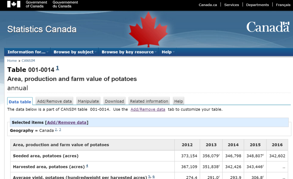
Statistics Canada download pages often provide the opportunity to modify the data structure and content before it is downloaded.
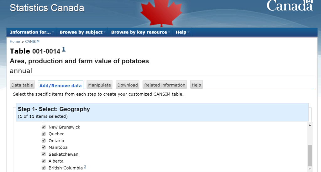
For example clicking on the [Add/Remove data] link provides options select different groupings of data by provinces. I choose to group data by provinces.
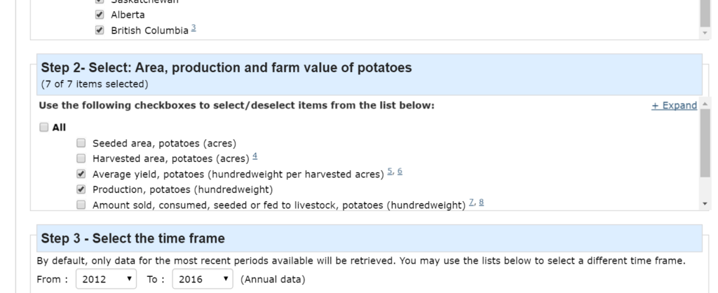
I also limited the content to only yield and production. There are other metrics available though they are often differing presentations of the data eg relative amounts by category etc.
I selected option to download the data as a csv formatted text file.
This csv file data had to be transformed before it could be used for analysis.
Statistics Canada often includes non-data text such as report titles and descriptions in the first rows of text files and footer notes in rows below the actual data.
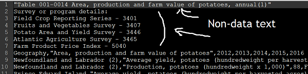
Before we can work with this data these title and footer rows have to be removed.
For this job I used Excel Power Query which can do the ETL. It can extract the data from the csv file, transform the data to a format that is amenable to analysis and load the data into a worksheet (or model) so it can be used for analysis.
Power Query has capabilities and features that match those of many more advanced ETL / integration software such as SSIS, Talend, Informatica, etc.
I have been encouraging and providing training to Excel users to move all of their ETL work in to Power Query. It brings the advanced capabilities of these tools to the relatively non technical desktop business user.
People too often copy and paste data from other sources into their Excel file.
With Power Query the original data file is a data source, and is linked into the Power Query, thus remains untouched and can simply be refreshed to get new or modified data at any time, providing that the columns and content remain unchanged. This makes it easy to get updated time sequence data as it comes available.
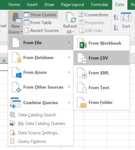
So back to our job. The first step was to link to the csv data file downloaded from Statistics Canada into Power Query by using New Query – From File – From CSV
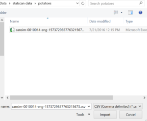
Select the data file and click Import.
Here is where we begin to bump into data file format challenges. Power Query can’t automatically determine file format because there are non-data text strings at top (report titles, descriptions) and bottom (footer notes).
I would like to encourage Statistics Canada and any other data provider to avoid doing this. A data file should be in a predictable tabular (CSV, tab separated) or other format (JSON, XML) without any other content that needs to be processed out.
But no problem. Power Query is equipped to deal with these situations.
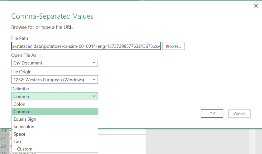
Power Query assumed this is csv file but the top rows of titles and descriptions do not have commas so it doesn’t split top rows into columns and as a result the split rows below are hidden.
One solution which I used was to go into the Power Query Source step settings to change the delimiter from Comma to Equals Sign. Since there are no equals signs the data is not split into columns and remains in one column that we can remove top and bottom non-data rows.
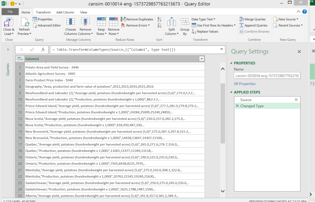
The Power Query Source step now looks like this.
= Csv.Document(File.Contents("C:\statscan data\potatoes\cansim-0010014-eng-1573729857763215673.csv"),[Delimiter="=", Encoding=1252])
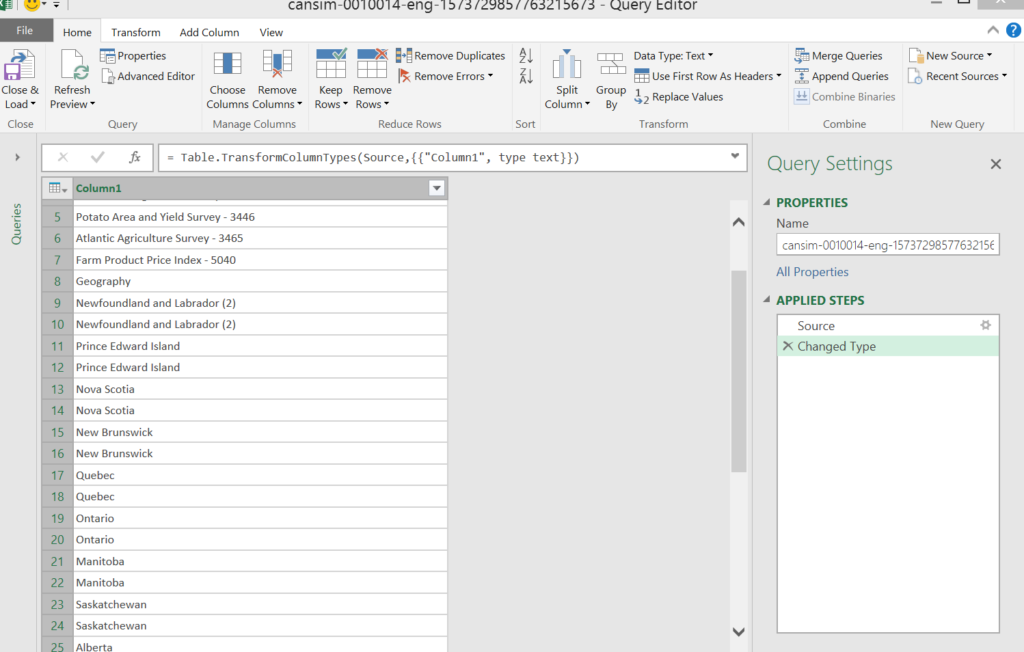
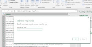
Now we can remove the non-data text from the data file. Select the Remove Rows – Remove Top Rows and enter the number of rows to remove (in this case it is top 7 rows are non-data rows).
= Table.Skip(#"Changed Type",7)
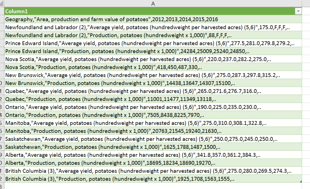
Do the same for the bottom rows but select Remove Rows – Remove Bottom Rows.
= Table.RemoveLastN(#"Removed Top Rows",12)
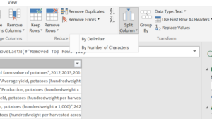
Now we can load the data to the worksheet and we will see one column of comma separated values which we just need to split to get nice columns of data.
Tell Power Query to split columns by comma.
= Table.SplitColumn(#"Removed Bottom Rows","Column1",Splitter.SplitTextByDelimiter(",", QuoteStyle.Csv),{"Column1.1", "Column1.2", "Column1.3", "Column1.4", "Column1.5", "Column1.6", "Column1.7"})
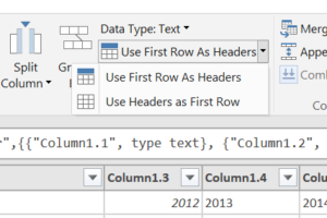
Also tell Power Query to use first row as headers. If the non-data text rows were not in the file Power Query would have done this automatically.
= Table.PromoteHeaders(#"Changed Type1")
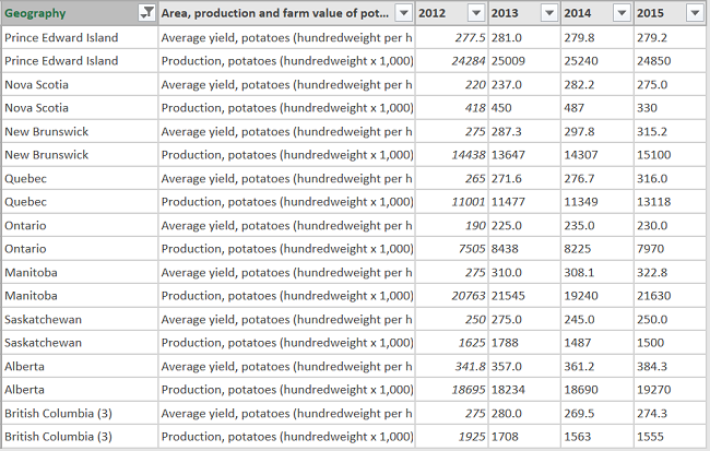
A key data transformation to get this data into a useful tabular format is to unpivot the years columns to rows. This is one of Power Query’s most useful transformations. Many data sources, especially in enterprise business, often have time series or other categories presented as columns but to do dimensional analysis these have to be unpivoted so they are in rows instead of columns.
Note that the Statistics Canada data formatting feature often includes moving time series to rows which would be similar transformation to this Power Query Unpivot.
Here is the pivoted data.
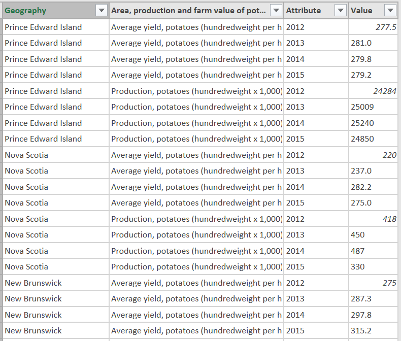
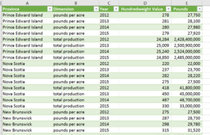
And here is the unpivoted data. This now gives us unique columns of data that can be used by any analytical software.
I also did some other things to clean up the data:
- Renaming column headers to be shorter, more readable.
- Changing the dimension values to shorter strings.
- Changing hundredweight values to pounds multiplying production values by 1000 to get full values.
- Filtered out Newfoundland because it was missing 2013, 2014, 2015 values.
- Removed the 2016 column which had no values.
Once loaded back to worksheet we now have nice clean dimensional data ready for us to begin working with in any analytical software. This can be used as data source for Tableau, Qlikview, Cognos, Birst, etc.
Lets take a quick look at the data using Excel Pivot Tables and Charts. Select this worksheet table and select Insert – Pivot Table to create a new pivot table like the one below.
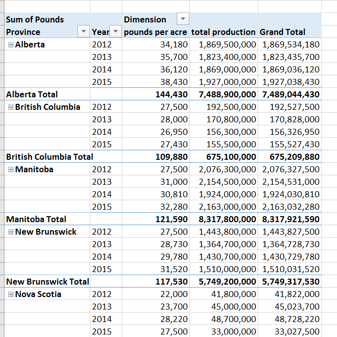
Select Insert Pivot Chart to create new pivot chart from this pivot table.
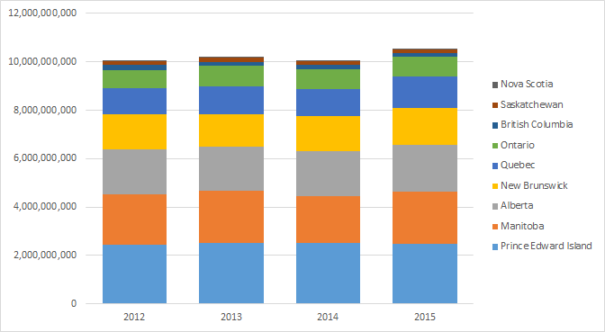
In this case I selected a stacked bar chart that show total Canadian potato production by province.
This does a good job of demonstrating relative contribution to total by province.
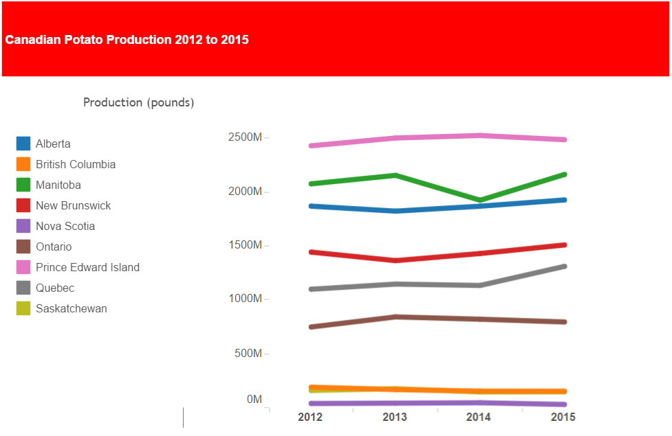
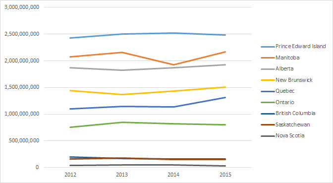
A stacked line chart does a better job of illustrating changes in production by provinces by year.
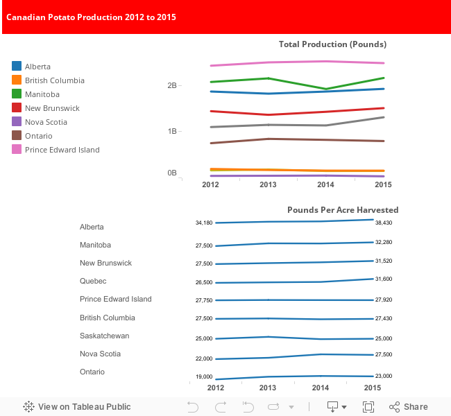
Here is a Tableau 9 report from the Power Query results.
Here is the complete Power Query M-code copied from the Power Query that gets and transforms the Statistics Canada raw csv data file into the transformed data set ready to be used in Excel Pivot Tables/Charts and Tableau or any other reporting tool.
let
    Source = Csv.Document(File.Contents("C:\Users\bb\Documents\Dropbox\Data\statscan data\potatoes\cansim-0010014-eng-1573729857763215673.csv"),[Delimiter="=", Encoding=1252]),
    #"Changed Type" = Table.TransformColumnTypes(Source,{{"Column1", type text}}),
    #"Removed Top Rows" = Table.Skip(#"Changed Type",7),
    #"Removed Bottom Rows" = Table.RemoveLastN(#"Removed Top Rows",12),
    #"Split Column by Delimiter" = Table.SplitColumn(#"Removed Bottom Rows","Column1",Splitter.SplitTextByDelimiter(",", QuoteStyle.Csv),{"Column1.1", "Column1.2", "Column1.3", "Column1.4", "Column1.5", "Column1.6", "Column1.7"}),
    #"Changed Type1" = Table.TransformColumnTypes(#"Split Column by Delimiter",{{"Column1.1", type text}, {"Column1.2", type text}, {"Column1.3", type number}, {"Column1.4", type text}, {"Column1.5", type text}, {"Column1.6", type text}, {"Column1.7", type text}}),
    #"Promoted Headers" = Table.PromoteHeaders(#"Changed Type1"),
    #"Removed Columns" = Table.RemoveColumns(#"Promoted Headers",{"2016"}),
    #"Filtered Rows" = Table.SelectRows(#"Removed Columns", each ([Geography] <> "Newfoundland and Labrador (2)")),
    #"Unpivoted Columns" = Table.UnpivotOtherColumns(#"Filtered Rows", {"Geography", "Area, production and farm value of potatoes"}, "Attribute", "Value"),
    #"Renamed Columns" = Table.RenameColumns(#"Unpivoted Columns",{{"Attribute", "Year"}, {"Area, production and farm value of potatoes", "Dimension"}, {"Geography", "Province"}, {"Value", "Hundredweight Value"}}),
    #"Changed Type2" = Table.TransformColumnTypes(#"Renamed Columns",{{"Hundredweight Value", type number}}),
    #"Replaced Value" = Table.ReplaceValue(#"Changed Type2","Average yield, potatoes (hundredweight per harvested acres) (5,6)","pounds per acre",Replacer.ReplaceText,{"Dimension"}),
    #"Replaced Value1" = Table.ReplaceValue(#"Replaced Value","Production, potatoes (hundredweight x 1,000)","production",Replacer.ReplaceText,{"Dimension"}),
    #"Added Custom" = Table.AddColumn(#"Replaced Value1", "Pounds", each if [Dimension] = "pounds per acre" then [Hundredweight Value] * 100 else if [Dimension] = "production" then [Hundredweight Value] * 100 * 1000 else null)
in
    #"Added Custom"