Introduction to Excel Power Query aka Power BI Query
What is Power Query? Power Query is an Microsoft tool for Excel that is used to do the following: Connect to a data source Extract data from source Transform the extracted data Load the transformed data into Excel This functionality is called ETL (Extract, Transform and Load). Why use Power Query? Excel already has another […]
Introduction to Excel Power Query aka Power BI Query Read More »