
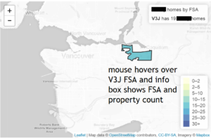
I have a Django web application that needed an interactive map with shapes corresponding to Canadian postal code FSA areas that were different colors based on how many properties were in each FSA. It ended up looking something like the screenshot below.
This exercise turned out to be relatively easy using the awesome open-source Javascript map library Leaflet.js.
I used this Leaflet.js tutorial as the foundation for my map.
One of the biggest challenges was finding a suitable data source for the FSAs. Chad Skelton (now former) data journalist at the Vancouver Sun wrote a helpful blog post about his experience getting a suitable FSA data source. I ended up using his BC FSA data source for my map.
Statistics Canada hosts a Canada Post FSA boundary files for all of Canada. As Chad Skelton notes these have boundaries that extend out into the ocean among other challenges.
Here is a summary of the steps that I followed to get my choropleth map:
1. Find and download FSA boundary file. See above.
2. Convert FSA boundary file to geoJSON from SHP file using qGIS.
3. Create Django queryset to create data source for counts of properties by FSA to be added to the Leaflet map layer.
4. Create Leaflet.js map in HTML page basically the HTML DIV that holds the map and separate Javascript script that loads Leaflet.js, the FSA geoJSON boundary data and processes it to create the desired map.
Find and download FSA boundary file.
See above.
Convert FSA boundary file to geoJSON from SHP file using qGIS.
Go to http://www.qgis.org/en/site/ and download qGIS. Its free and open source.
Use qGIS to convert the data file from Canada Post or other source to geoJSON format. Lots of blog posts and documentation about how to use qGIS for this just a Google search away.
My geoJSON data source looked like this:
var bcData = {
    "type": "FeatureCollection",
    "crs": { "type": "name", "properties": { "name": "urn:ogc:def:crs:EPSG::4269" } },
    "features": [
    { "type": "Feature", "properties": { "CFSAUID": "V0A", "PRUID": "59", "PRNAME": "British Columbia \/ Colombie-Britannique" }, "geometry": { "type": "MultiPolygon", "coordinates": [ [ [ [ -115.49499542, 50.780018587000029 ], [ -115.50032807, 50.77718343600003 ], [ -115.49722732099997, 50.772528975000057 ], [ -115.49321284, 50.770504059000075 ], [ -115.49393662599999, 50.768143038000062 ], [ -115.50289288699997, 50.762270941000054 ], [ -115.50846411599997, 50.754243300000041 ], [ -115.5104796, 50.753297703000044 ], [ -115.51397592099994, 50.748953800000038 ], [ -115.51861431199995, 50.745737989000077 ], [ -115.52586378899997, 50.743771099000071 ], [ -115.53026371899995, 50.74397910700003 ], [ -115.53451319199996,
Create Django queryset to create data source for counts of properties by FSA to be added to the Leaflet map layer.
I used a SQL query in the Django View to get count of properties by FSA.
This dataset looks like this in the template. These results have only one FSA, if it had more it would have more FSA / count pairs.
Below is code for the Django view query to create the fsa_array FSA / counts data source.
cursor = connection.cursor()
    cursor.execute(
    "select fsa, count(*) \
    from properties \
    group by fsa \
    order by fsa;")
    fsas_cursor = list(cursor.fetchall())

    fsas_array = [(x[0].encode('utf8'), int(x[1])) for x in fsas_cursor]
My Javascript largely retains the Leaflet tutorial code with some modifications:
1. How the legend colors and intervals are assigned is changed but otherwise legend functions the same.
2. Significantly changed how the color for each FSA is assigned. The tutorial had the color in its geoJSON file so only had to reference it directly. My colors were coming from the View so I had to change code to include new function to match FSA’s in both my Django view data and the geoJSON FSA boundary file and return the appropriate color based on the Django View data set count.
var fsa_array = [["V3J", 19]];

var map = L.map('map',{scrollWheelZoom:false}).setView([ active_city_center_lat, active_city_center_lon], active_city_zoom);

map.once('focus', function() { map.scrollWheelZoom.enable(); });

var fsa_array = fsas_array_safe;

L.tileLayer('https://api.tiles.mapbox.com/v4/{id}/{z}/{x}/{y}.png?access_token=pk.eyJ1IjoibWFwYm94IiwiYSI6ImNpandmbXliNDBjZWd2M2x6bDk3c2ZtOTkifQ._QA7i5Mpkd_m30IGElHziw', {
    maxZoom: 18,
    attribution: 'Map data ©' + OpenStreetMap CC-BY-SA' + 'Imagery ©' + 'Mapbox'
    id: 'mapbox.light'
}).addTo(map);

// control that shows state info on hover
var info = L.control();

info.onAdd = function (map) {
    this._div = L.DomUtil.create('div', 'info');
    this.update();
    return this._div;
};

info.update = function (props) {
    this._div.innerHTML = (props ?
        '' + props.CFSAUID + ' ' + getFSACount(props.CFSAUID) + ' lonely homes'
        : 'Hover over each postal area to see lonely home counts to date.');
};

info.addTo(map);

// get color
function getColor(n) {
    return n > 30 ? '#b10026'
           : n > 25 ? '#e31a1c'
           : n > 25 ? '#fc4e2a'
           : n > 20 ? '#fd8d3c'
           : n > 15  ? '#feb24c'
           : n > 10  ? '#fed976'
           : n > 5  ? '#ffeda0'
           : n > 0  ? '#ffffcc'
           : '#ffffff';
}

function getFSACount(CFSAUID) {
    var fsaCount;
    for (var i = 0; i < fsa_array.length; i++) {
        if (fsa_array[i][0] === CFSAUID) {
            fsaCount = ' has ' + fsa_array[i][1];
            break;
        }
    }
    if (fsaCount == null) {
         fsaCount = ' has no ';
    }
    return fsaCount;
}

function getFSAColor(CFSAUID) {
    var color;
    for (var i = 0; i < fsa_array.length; i++) {
    if (fsa_array[i][0] === CFSAUID) {
        color = getColor(fsa_array[i][1]);
        //console.log(fsa_array[i][1] + '-' + color)
        break;
        }
    }
    return color;
}

function style(feature) {
    return {
        weight: 1,
        opacity: 1,
        color: 'white',
        dashArray: '3',
        fillOpacity: 0.7,
        fillColor: getFSAColor(feature.properties.CFSAUID)
    };
}

function highlightFeature(e) {
    var layer = e.target;
    layer.setStyle({
        weight: 2,
        color: '#333',
        dashArray: '',
        fillOpacity: 0.7
    });

    if (!L.Browser.ie && !L.Browser.opera) {
        layer.bringToFront();
    }

    info.update(layer.feature.properties);
}

var geojson;

function resetHighlight(e) {
    geojson.resetStyle(e.target);
    info.update();
}

function zoomToFeature(e) {
    map.fitBounds(e.target.getBounds());
}

function onEachFeature(feature, layer) {
    layer.on({
        mouseover: highlightFeature,
        mouseout: resetHighlight,
        click: zoomToFeature
    });
}

geojson = L.geoJson(bcData, {
    style: style,
    onEachFeature: onEachFeature
}).addTo(map);

var legend = L.control({position: 'bottomright'});

legend.onAdd = function (map) {

    var div = L.DomUtil.create('div', 'info legend'),
        grades = [0, 1, 5, 10, 15, 20, 25, 30],
        labels = [],
        from, to;

    for (var i = 0; i < grades.length; i++) {
        from = grades[i];
        if (i === 0) {
            var_from_to = grades[i];
            var_color = getColor(from);
        } else {
            var_from_to =  from + (grades[i + 1] ? '–' + grades[i + 1] : '+') ;
            var_color = getColor(from + 1);
        }

        labels.push(
            ' ' +
             var_from_to);
    }

    div.innerHTML = labels.join('');
    return div;
};

legend.addTo(map);
That is pretty much all there is to creating very nice looking interactive free open-source choropleth maps for your Django website application!